Part 2 traces the evolution of transformer architecture from vanilla transformers to modern LLMs.

This article is for anyone who understands the basic attention mechanism and wants to see why serving a large language model gets expensive as conversations grow. You will learn how KV Cache removes redundant computation, how to estimate its memory cost, and why that cost pushed researchers toward MQA, GQA, and MLA.

What Query, Key, and Value actually do

A simple way to read attention is as a search system. The Query (Q) is the question. The Key (K) tells you what each token represents, so the model can judge whether that token is relevant to the query. The Value (V) is the information actually retrieved when a token turns out to be relevant.

This division of labor explains why positional information in RoPE is applied mainly to Q and K: attention decides which tokens should interact through the Q-K relationship. KV Cache, however, solves a different problem entirely.

The repetition problem in autoregressive generation

During inference, an LLM generates one token at a time. At every new step, the newly generated token must attend to all previous tokens. Suppose the model has already produced: The → name → is → Naimish. When generating the next token, it needs the Key and Value representations of all prior tokens.

Without caching, the growing sequence forces the model to recompute K and V for tokens it has already processed. At step one, it computes K₁ and V₁ for "The." At step two, it computes K₁ and V₁ again, then adds K₂ and V₂. At step three, it recomputes K₁ and V₁, recomputes K₂ and V₂, then adds K₃ and V₃. The Keys and Values for "The" and "name" have already been calculated, yet they keep being calculated again.

Compute the past once, then reuse it

The fix is to store previously calculated K and V in memory instead of discarding them. When the next token arrives, the model calculates only the new K and V and appends them to the existing cache. Conceptually: after step one the cache holds [K₁, V₁]; after step two it holds [K₁, K₂] and [V₁, V₂]; after step three it holds [K₁, K₂, K₃] and [V₁, V₂, V₃].

The model reuses the previously computed representations rather than recalculating the past. This significantly reduces redundant computation during autoregressive inference and is one of the most important techniques for making LLM generation efficient. But the optimization introduces a new question: if we keep storing K and V for every previous token, how much GPU memory will the cache consume as context grows?

How Q, K, and V are computed

During training, the model learns its parameters, including the projection matrices that generate Q, K, and V. Once training is complete, these weights are fixed during inference, and inference uses those trained weights to calculate Q, K, and V for input tokens.

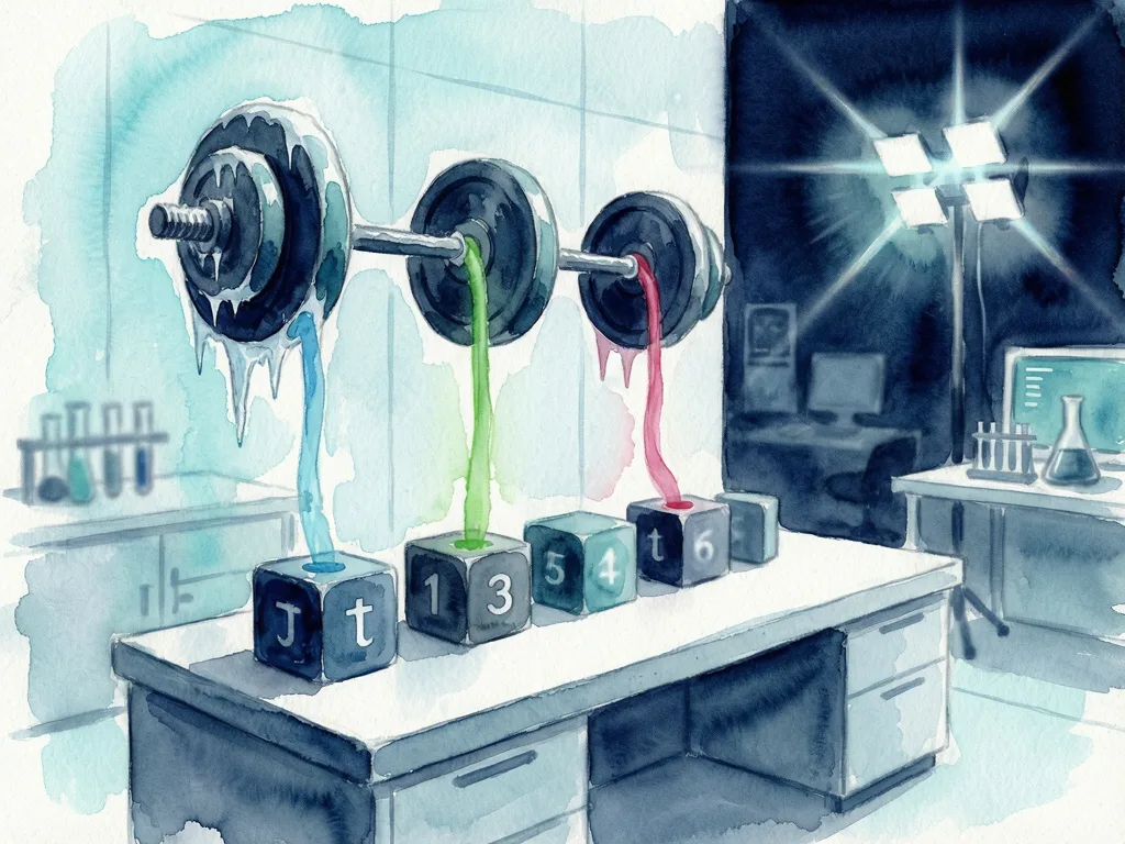
Take a four-token input: The, name, is, naimish. For simplicity, assume each token is represented by a 3-dimensional embedding, giving an input matrix X of shape 4 × 3, where 4 is the number of tokens and 3 is the embedding dimension. The Transformer contains three learned projection matrices: Wq for Query, Wk for Key, and Wv for Value. In this simplified example, Wq is a 3 × 3 matrix with rows [0.12, 1.3, 8.4], [2.4, 5.7, 2.9], and [1.2, 7.4, 1.7]; Wk and Wv are defined similarly. These matrices were learned during training and stay fixed during inference.

We then calculate Q = XWq, K = XWk, and V = XWv. With X at 4 × 3 and each projection at 3 × 3, Q, K, and V each come out at 4 × 3. In a real multi-head Transformer, these projections are divided across attention heads, but the basic idea is unchanged.

From Q, K, V to attention scores

To decide which tokens should receive more attention, the model computes the similarity between every Query and every Key using the dot product: Attention Scores = QKᵀ. It then scales the scores by the square root of the Key dimension, giving QKᵀ / √dₖ, and applies Softmax to obtain attention weights. Finally, the weights are multiplied by the Value matrix. The complete scaled dot-product attention formula is Attention(Q, K, V) = softmax(QKᵀ / √dₖ)V.

The flow matters: Q × Kᵀ measures how relevant each token is, Softmax turns that into attention weights, and multiplying by V produces the context or attended representation. This is exactly where KV Cache pays off. The Query for the newly generated token must interact with the Keys of all previous tokens, but those previous Keys have already been calculated. Instead of recomputing them, the model reuses them from the cache. Only the new token's K and V need to be calculated and appended.

The memory bill

KV Cache solves one major problem, repeatedly recomputing the Keys and Values of previous tokens, but it creates another: all those Keys and Values now sit in GPU memory, and the cache grows with the context. Ten generated tokens mean ten sets of K and V. One thousand tokens mean one thousand sets. One hundred thousand tokens mean one hundred thousand sets.

The numbers get serious quickly. For a 7B-parameter model with 32 layers, 32 attention heads, head dimension d = 128, running in FP16 with a batch size of 1, the KV Cache consumes roughly 1 GB at 4K tokens, about 8 GB at 32K tokens, and around 32 GB at 128K tokens. At 128K tokens, the cache alone can require about 32 GB of VRAM, before accounting for model weights and other runtime requirements. That is why KV Cache becomes a serious memory bottleneck as context length increases. In short, it trades computation for memory.

Why the cache scales the way it does

Consider a Transformer with L layers, H_KV Key-Value heads, head dimension d, and context length T. For every layer and every token, both K and V must be stored. Ignoring batch size, data type, and implementation details, the approximate number of cached values is proportional to 2 × L × T × H_KV × d_head, where the 2 comes from storing both K and V.

The practical reading: KV Cache size scales with context length × number of KV heads × head dimension × number of layers. As context length rises, the cache can become extremely large. Notice also that cache memory is directly proportional to the number of Key-Value heads, which means reducing K/V heads directly reduces inference memory. Multi-Head Attention (MHA) uses many KV heads, Grouped-Query Attention (GQA) uses fewer, and Multi-Query Attention (MQA) uses one.

Why Multi-Head Attention is the expensive case

In standard MHA, every attention head has its own Query, Key, and Value projections: Head 1 → Q₁, K₁, V₁; Head 2 → Q₂, K₂, V₂; and so on through Head H → Qₕ, Kₕ, Vₕ. During autoregressive inference, the model must therefore cache K₁, V₁ through Kₕ, Vₕ for every previous token and every Transformer layer.

The Query vectors are not the problem. The Query of the new token is computed and used at each decoding step. The major memory cost comes from storing the historical K and V for all tokens. That raises the question that reshaped attention design: do we really need a separate Key and Value cache for every attention head?

What comes next

KV Cache is one of the simplest but most important optimizations for efficient LLM inference. It replaces a computation problem with a memory problem, and that memory problem gets worse as context length, layer count, and KV head count grow. It becomes especially acute with MHA, where every attention head maintains its own Key and Value representations.

The follow-on question, whether every Query head truly needs its own K and V, led to more memory-efficient architectures: MQA, then GQA, and eventually more sophisticated approaches such as MLA (Multi-Head Latent Attention). Reducing KV-cache memory is only one part of efficient attention, however. The actual computation and memory movement in attention also became a major bottleneck, which led to techniques such as Flash Attention and other efficient-attention mechanisms.

The evolution is not about replacing the Transformer overnight. Researchers kept asking whether attention can stay strong while becoming faster, cheaper, and more memory-efficient. That is the thread to follow in the next part.